7 years, 1 month ago
Eighteen Months of RL Research at Google Brain in Montreal
Back in the summer of 2017, in-between a few farewell vacations around Europe, I became a (then-remote) member of the newly-formed Google Brain team in Montreal. My home office offered a stunning view of Belsize Park in northern London, and hosted the entirety of Google Montreal’s RL group: yours truly.
Since then, I’ve moved to a different continent, and between AI residents, student researchers, and full-time Googlers, the team has expanded considerably (and continues to do so: Marlos C. Machado joined us this week). In hindsight, 2018 was an incredibly productive year. This blog post looks back at our scientific output during the period to provide a bird’s eye view of the RL research at Google Brain in Montreal, of the amazing collaborations we’ve taken part in, and to give a sense for what lies a short distance ahead for us.
Distributional reinforcement learning
“That’s all fine. But why does it work?”
In reinforcement learning, the distributional perspective suggests that we should predict the distribution of random returns, instead of their expected value (Bellemare, Dabney, Munos, ICML 2017). However, most distributional agents still behave by distilling action-value distributions back down to their respective expected values, then selecting the action with the highest expected value. Predict, then distill. So why does it perform so well in practice?
To answer this question, we developed a formal language for analyzing distributional RL methods, in particular sample-based ones (Rowland et al., AISTATS 2018). This formalization led us to discover that the original distributional algorithm (called C51) implicitly minimizes a distance between probability distributions called the Cramér distance. But some of our results suggest distributional algorithms should minimize the Wasserstein distance between distributions, not the Cramér distance. We (by we, I really mean Will Dabney) re-vamped most of C51 using a technique called quantile regression, which does in part minimize the Wasserstein distance. The resulting agent (this one is called QR-DQN) exhibits strong performance on the Atari 2600 benchmark (Dabney et al., AAAI 2018). Another exciting result is Mark Rowland’s recent discovery of an interesting mismatch between statistics and samples in distributional RL, which explains why these algorithms work and others are doomed to failure (Rowland et al., 2019).
Following Mark’s analysis of C51, we derived a distributional algorithm from first principles – in this case using the Cramér distance, which is easier to work with. The goal was to create a distributional algorithm that explicitly performs gradient descent on a distributional loss (something neither C51 nor QR-DQN does). The result is an algorithm we’ve named S51 (Bellemare et al., AISTATS 2019); The ‘S’ stands for ‘signed’, because the algorithm may output what are effectively negative probabilities. Thanks to its relatively simplicity, we were able to show that S51 has convergence guarantees when combined with linear function approximation. Along the way, we also gathered evidence that there are pathological examples where the predict-and-distill approach is a worse approximation than directly predicting expected values, a natural consequence of what one reviewer called being “more prone to model misspecification”.
We’ve since shown that predict-and-distill is in fact ineffective when combined to tabular representations, and confirmed that it is likely to perform worse than expected RL when combined with linear representations (Lyle, Castro, Bellemare, AAAI 2019). This has let us rule out common explanations that do not depend on the choice of representation, such as “distributional RL reduces variance” or “averaging distributional predictions leads to more accurate value estimates”. Somewhat misquoting Mr. Holmes, once you’ve eliminated the impossible, what remains must be the truth: it seems that distributional RL becomes useful once combined with deep networks.
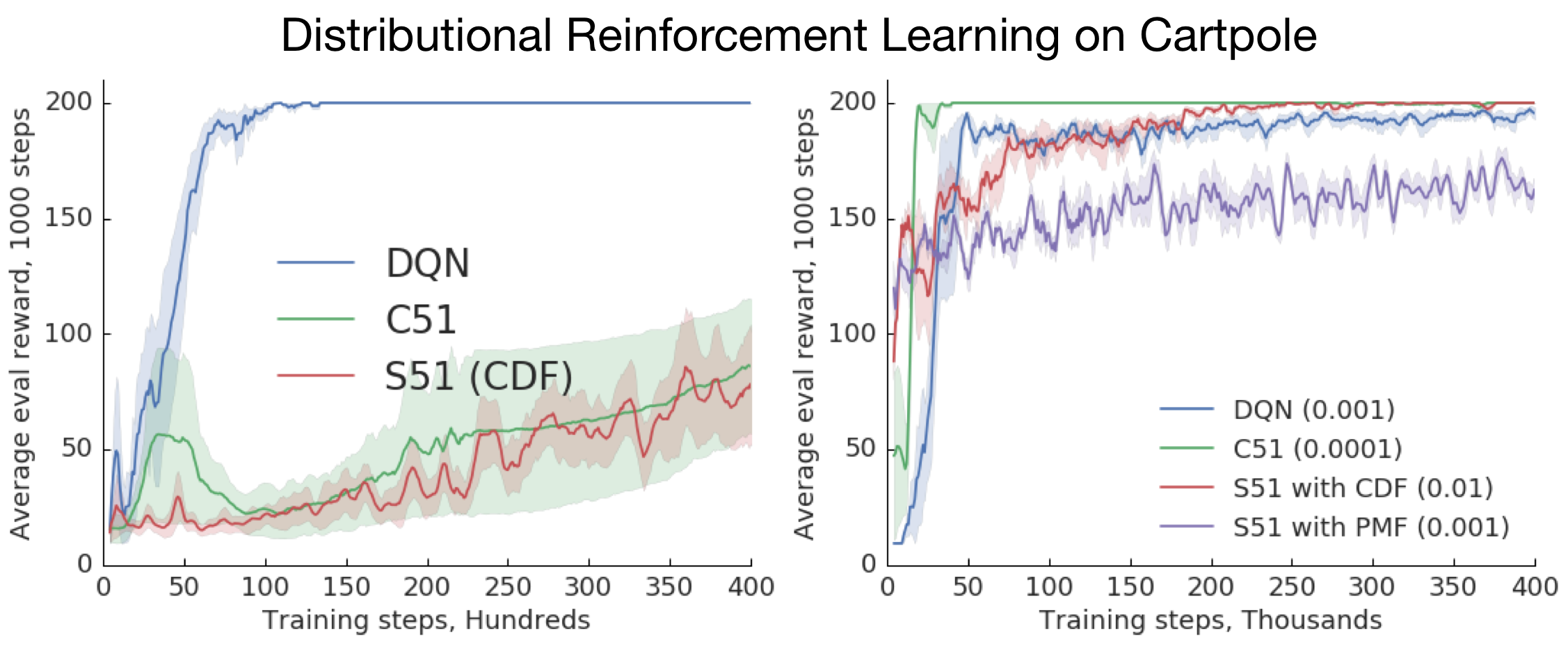
To collect further evidence for this, we trained agents on the Cartpole domain, either using a fixed, low-dimensional representation (an order 1 Fourier basis) or a comparable deep network. The results (summarized in the plots below) are rather telling: with a fixed representation, the distributional methods perform worse than expectation-based methods; but with a deep representation, they perform better. The paper also shows that Cramér-based methods should output cumulative distribution functions, not probability mass functions (PMFs).
As a deep learning practitioner, it’s natural to conclude that distributional RL is useful because “it helps learn better representations”. But what does that mean, formally? And how does one prove or disprove this kind of statement? These questions led us to work on a very hot topic: representation learning for reinforcement learning.
Representation learning
Last summer, Will Dabney and I designed what we call an “apple pie” experiment for representation learning in RL: a no-frills setup to study what it means to learn a good representation. The experiment involves 1) a synthetic environment (the four-room domain) in which we 2) train a very large deep network 3) to make a variety of predictions. We define a representation as a mapping from states to d-dimensional feature vectors, which are in turn linearly mapped to predictions. In all experiments, d is smaller than the number of states. This setup lets us answer questions such as: “What is the resulting representation when we train the network to predict X?”, where X might be a value function, a value distribution, or some auxiliary tasks.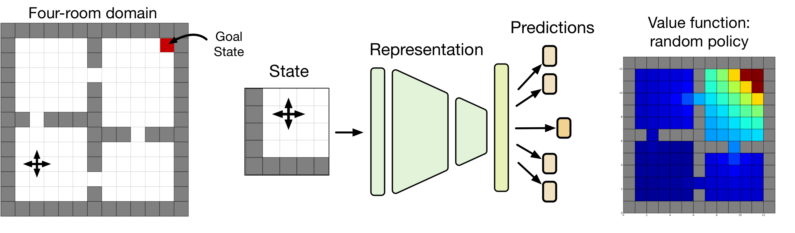
By poking and prodding at our little problem, we realized we could formulate an optimality criterion for representations. This criterion states that an optimal representation should minimize the approximation error over all “achievable” value functions, where by “achievable” I mean “generated by some policy” (Bellemare et al., 2019). In fact, one only needs to consider a very special subset of such value functions, which we call adversarial value functions (AVFs) to reflect the minimax flavour of the optimality criterion. The results are also interesting because the arguments are mostly geometric in nature. Along the way, we found that the space of value functions itself is highly structured: it is a polytope, albeit one with some unintuitive characteristics (Dadashi et al, 2019).
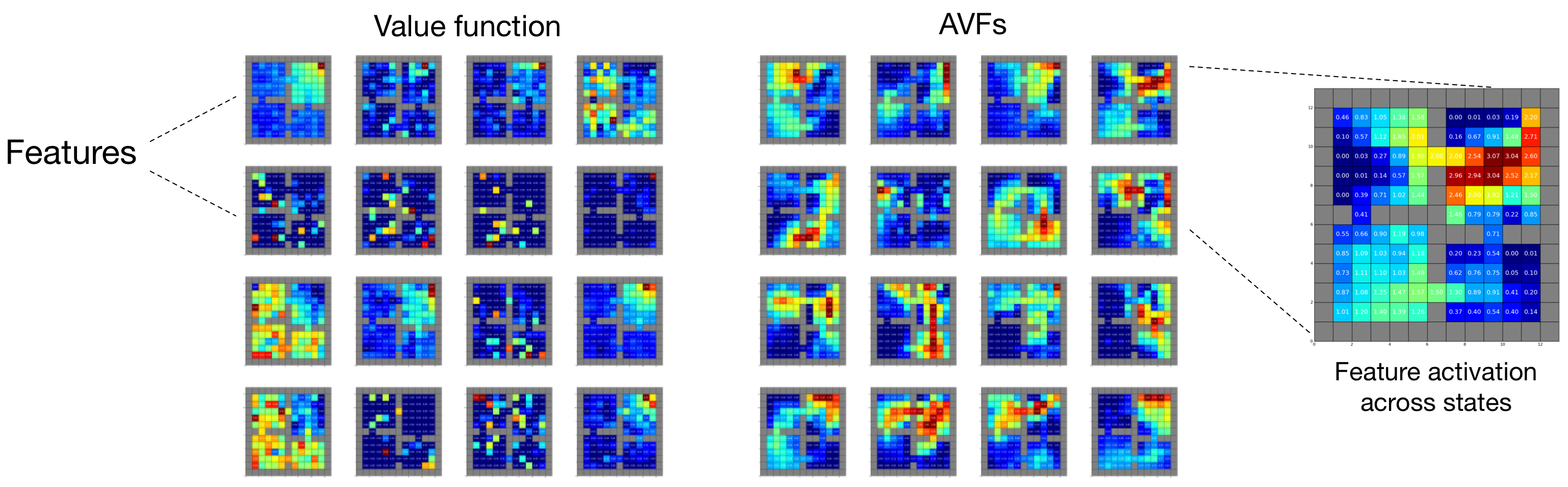
We visualize the effect of the method using a kind of “FMRI for representations” (above; code credits to Marlos C. Machado). Here, each cell depicts the normalized activation of a feature as a function of the input state. The figure compares what happens when the network is trained to predict either a single value function or a large set of AVFs. The value-only representation is somewhat unsatisfying: individual features are either inactive across states, or copies of the predicted value function; there is also noise in the activation patterns. The AVF method, by contrast, yields beautiful structure.
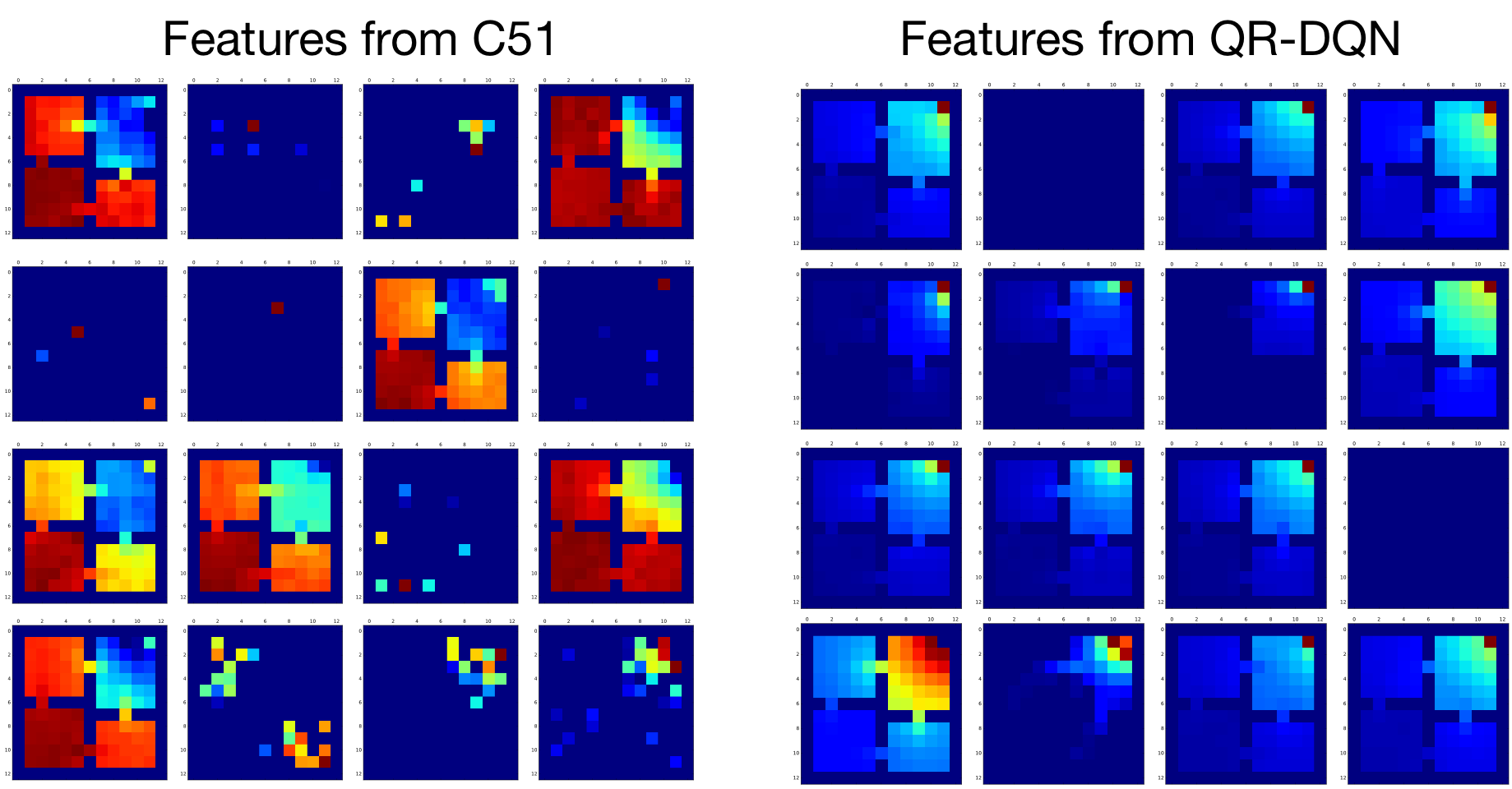
We can use the same tools to confirm that distributional RL does learn richer representations. Below is a visualization of the features learned when predicting the value distribution of the random policy using C51 (left), or using QR-DQN (right). The features learned by quantile regression offer a gradation of responses, from highly peaked around the goal (2nd from left, bottom row) to relatively diffuse (top right). Both sets of features are more structured than when we just learn the value function (previous figure, left).
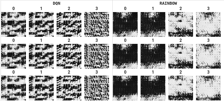
Complementary to these results, we visualized the activation of hidden units in Atari 2600 game-playing agents. These form part of a fantastic collaboration on an “Atari Zoo” with Pablo Samuel Castro, Felipe Such, Joel Lehman & many others (Such et al., Deep RL Workshop at NeurIPS, 2018). To highlight but one result, the convolutional features learned by a distributional algorithm (Hessel et al.’s extension of C51, called Rainbow) are often more detailed and complex than those learned by the non-distributional DQN, as the following example from the game Seaquest shows:
Also hot off the press, we’ve found that predicting value functions for multiple discount rates is also a simple and effective way to produce auxiliary tasks in Atari 2600 games (Fedus et al., 2019).
The evidence leaves no doubt that different RL methods yield different representations, and that complex interactions occur at the interface between deep and reinforcement learning. With some luck, the coming year will also shed some light on the relationship between these representations and an agent’s empirical performance.
Software
If you attended one of my talks in the last year, you may have seen me present the following:
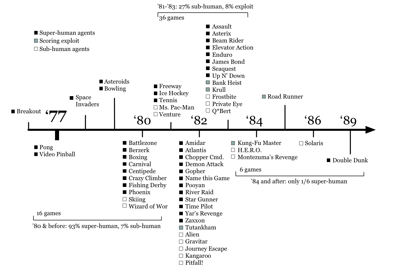
The timeline arranges the 60 games available via the Arcade Learning Environment chronologically, based on their release date. Each title is labelled with a (subjective) estimate of the performance of our best learning agents: superhuman ◼, subhuman (empty), and finally score exploit (grey) for games in which the AI achieves high scores without playing the game the intended way. The timeline shows that there are proportionally more “superhuman” labels in the early games than the latter ones. This, I argue, gives evidence that early games are easier than later ones, in part because of a shift in video game experience: from reactive (Pong) to cognitive (Pitfall!).
Note that the timeline is from mid-2017 and a little dated now; adjusted to take into account the kind of big performance leaps we’ve seen on e.g. Montezuma’s Revenge via imitation learning (Hester et al., 2017; Aytar et al., 2018) and nonparametric schemes (Ecofett et al., 2019), there might be few empty boxes left. Given how instrumental the ALE was in driving the revival of deep RL research, it makes sense that the RL community should now be actively seeking the “next Atari”.
But the graph helps me make another point: the ALE is now a mature benchmark, to be treated differently from emerging challenges. To quote Miles Brundage, Atari game-playing is “alive as an RL benchmark if one cares about sample efficiency”. Deep reinforcement learning itself is also maturing: for a nice overview of current techniques, see Vincent François-Lavet’s review (2019), to which I contributed. After heady early successes, Deep RL might be ready to go back to basics.
One outcome of this maturing is a second iteration of the ALE paper, led by my then-student Marlos C. Machado and bundled with a new code release which unlocks additional difficulty levels (“flavours”) that should prove quite useful to transfer learning research (Machado et al., 2018). There are really too many good things in this paper to list, but top of mind is a discussion on how to evaluate learning Atari-playing algorithms with reproducibility and fairness in mind. A nice example of how the community picked up on this can be seen in the Twitter-eddies of the Go-Explore blog post, where after some discussion the authors went back to evaluate their method on our recommended “sticky actions” evaluation scheme (here is one tweet by Jeff Clune, if you’re curious).
Last August we also released our open-source RL framework, Dopamine (white paper: Castro et al., 2018). With Dopamine we wanted to start simple and stick to a small core set of features useful to RL research. Consequently, the first version of the framework consists of about a dozen Python files, and provides a single-GPU, state-of-the-art Rainbow agent for the ALE. Dopamine 2.0 (Feb 6th blog post by Pablo Samuel Castro) expands this first version to support discrete-action domains more generally. Almost all of our recent RL work uses Dopamine.
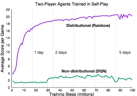
Last but not least, in collaboration with DeepMind we also recently released a new research platform for AI methods based on the highly popular card game Hanabi (Bard et al., 2019). Hanabi is unique because combines cooperative (not competitive!) play with partial observability. The code contains, among other things, a Dopamine-based agent so you can get started right away. I’ve already said much more about this in a different blog post, but will conclude by saying that I think this is one of the most interesting problems I’ve worked on for a while. Oh, and by the way: there seems to be a big performance gap between distributional and non-distributional RL, as the learning curve below shows. Small mystery.
Wrapping it up
This post doesn’t discuss exploration, even though the topic remains dear to my heart. Of note, with Adrien Ali Taiga we’ve made some progress towards understanding how pseudo-counts help us explore (Ali Taiga, Courville, Bellemare, 2018). It’s been great to see the RL community rise to the challenge and tackle hard exploration problems such as Montezuma’s Revenge. Although epsilon-greedy and entropy regularization still reign supreme in practice, I think we’re not very far from integrated solutions that significantly improve our algorithms’ sample efficiency.
Downtown Montreal might not quite offer the same views as North London, but the research is definitely no less exciting. Montreal and Canada are home to many of the world’s best researchers in deep and reinforcement learning and it’s been a pleasure to interact with so much talent, locally and across the Google Brain team.
Comments
Wei 7 years, 1 month ago
Wow very good post for your recent work.
Link | ReplyNew Comment